Diagnosing the Scheduler Timeout Error

This blog describes on - Diagnosing the Scheduler Timeout Error

When you run some huge bigsql queries or running many concurrent queries, sometimes you may get scheduler error. But when you rerun it, it will return the results.

In the db2diag log, you will see the error

2018-10-22-15.54.09.353224+540 I56948911015      LEVEL: Error
PID    : 29917               TID : 70312999533568 PROC : db2sysc 0
INSTANCE: bigsql              NODE : 000          DB  : BIGSQL
APPHDL : 0-2278              APPID: *1.bigsql.199921064012
AUTHID : BIGSQL              HOSTNAME: testcluster234.ibm.com
EDUID  : 228                 EDUNAME: db2agent (BIGSQL) 0
FUNCTION: DB2 UDB, base sys utilities, sqeBigSqlSchedulerInternal::registerQuery, probe:2690
MESSAGE : ZRC=0xFFFFEBB1=-5199
         SQL5199N The statement failed because a connection to a Hadoop I/O
         component could not be established or maintained. Hadoop I/O
         component name: "". Reason code: "". Database partition number: "".

DATA #1 : String, 140 bytes
Transport Exception occurred. The BigSql Scheduler service may not be running or the scheduler client request timeout may not be sufficient.

If you get the error,


 1) You need to check whether the scheduler is running.

                       $BIGSQL_HOME/bin/bigsql status -scheduler


2) If the scheduler is running, then you may need to check the time taken for scanning metadata & registerQueryNew. To get the time, you need to check the /var/ibm/bigsql/logs/bigsql-sched-recurring-diag-info.log

 [requestScanMetadata]
    top (5) max elapsed times:
      time= 4363; info= [TableSchema(schName:<schema>, tblName:<tablename>,         impersonationID:bigsql)]
      time= 2339; info= [TableSchema(schName:<schema>, tblName:<tablename>, impersonationID:user_tyre)]
      time= 32; info= [TableSchema(schName:<schema>, tblName:<tablename>, impersonationID:bigsql)]
    elapsed-time-range-in-millis and frequency-of-calls-in-that-range:
      range= 0-10; freq= 0
      range= 10-100; freq= 1
      range= 100-1000; freq= 0
      range= 1000-10000; freq= 2
      range= 10000-100000; freq= 0
      range= 100000-1000000; freq= 0
      range= 1000000-9223372036854775807; freq= 0
    
[registerQueryNew]
    top (5) max elapsed times:
      time= 448892; info= schema.tablename;
      time= 245079; info= schema.tablename;
      time= 204996; info= schema.tablename;
      time= 152660; info= schema.tablename;
      time= 151576; info= schema.tablename;
    elapsed-time-range-in-millis and frequency-of-calls-in-that-range:
      range= 0-10; freq= 71
      range= 10-100; freq= 18
      range= 100-1000; freq= 16
      range= 1000-10000; freq= 6
      range= 10000-100000; freq= 13
      range= 100000-1000000; freq= 9
      range= 1000000-9223372036854775807; freq= 0
    
You need to check the max time taken during the time when query failed. In above example, the max time is 448892 millisecond ( 7.48 mins).

Check the timeout set for the property (scheduler.client.request.IUDEnd.timeout & scheduler.client.request.timeout) in /usr/ibmpacks/current/bigsql/bigsql/conf/bigsql-conf.xml.

The default values are scheduler.client.request.timeout = 360000 (6 Mins) & scheduler.client.request.IUDEnd.timeout = 600000 (10 Mins)

  <property>
    <name>scheduler.client.request.IUDEnd.timeout</name>
    <value>600000</value>
    <description>
      Scheduler clients will wait for scheduler to respond for
      these many milli-seconds before timing out during RPC for
      finalizing Insert/Update/Delete.
      For Inserting/Updating/Deleting very large dataset,
      this many need to be adjusted.
    </description>
  </property>
 
  <property>
    <name>scheduler.client.request.timeout</name>
    <value>3600000</value>
    <description>
      Scheduler clients will wait for scheduler to respond for
      these many milli-seconds before timing out during any RPC
      call other than finalizing Insert/Update/Delete.
      For query over very large dataset, this many need to be adjusted.
    </description>
  </property>

As per the logs the query is taking 7.48 mins but the timeout we set in property is 6 mins. So we need to increase the timeout of property higher than the max timeout in the logs. You can change the timeout to 720000 (12 mins) and restart the BigSQL.

If you are using BigSQL 5.0.2 or above, you can do it from Ambari UI or you need to change it from /usr/ibmpacks/current/bigsql/bigsql/conf/bigsql-conf.xml

Data Science Experience - Exploratory Analysis using Python

The below blog provides various exploratory analysis on the dataset to get insight on data. As an example, I have taken the Titanic dataset from Kaggle ( Titanic DataSet )

The code is generalized for other dataset also. You can use the script for other dataset with minimal changes.


The complete python code is available in my github

Download the code from github and run the pyton script.

 

Output Generated

 

Sample output is uploaded to output folder.

1) 1_initial_data_analysis.txt

Provides an overview of No# of Attributes, Name of the Attributes, Type of Attribute, Mean/Max/Range for each Attributes, Attributes with no# of missing values, Possible categorial Attributes, Unique value for these categorial values etc.

Instance Count :  891
Attribute count (X,y) :  12
Attribute Names (X,y) :  ['PassengerId', 'Survived', 'Pclass', 'Name', 'Sex', 'Age',

 'SibSp', 'Parch', 'Ticket', 'Fare', 'Cabin',   'Embarked']

Most likely cataegorial values : ['Survived', 'Pclass', 'Sex', 'Age', 'SibSp', 

'Parch', 'Embarked']
Most likely **Non cataegorial values : ['PassengerId', 'Name', 'Ticket', 'Fare',

 'Cabin']

Sum of Missing Values for each attributes : 
    PassengerId      0
    Age            177
    Cabin          687
    Embarked         2

Unique values for cataegorial column :  Survived [0 1]
Unique values for cataegorial column :  Pclass [3 1 2]

 Refer the file for detailed output.

2) Histogram and Box ploting of all attributes in a single image to get the overall view of data

Histogram plotting of all Attributes

Box plotting of all Attributes

    
 
3) Ploting the Density and box plot with various additional information on catagorial attributes

Plotting of Attributes - Age

Plotting of Attributes - Fare

You can refer the ploting for other catagorial attributes under output/4_*_density_box_plot.png


4) Ploting the Categorial Attributes grouped by Target Attribute

Plotting of Age grouped by Survived

Plotting of Pclass grouped by Survived

You can refer the ploting for other catagorial attributes under   
                                                                          output/5_*_GroupBy_Survived_Histogram_plot.png


5) Pairwise plotting of Attribute

Pairwise plotting of Attributes

6) Ploting the Attributes by generalized values

Ploting Age_group

Plotting Cabin_group

 
 
7) Ploting generalized Attributes with respect to Target attribute

Ploting Age_group with Survived

Plotting Cabin_group with Survived

 

8) 9_GroupBy_Attribute_based_on_Target.txt

The file records provides the count of each attribute with respect to Target attribute.

Group by on Attribute : Sex
Dictionary Mapping : {'male': 0, 'female': 1}
    Sex  count  Survived
    0    0    468         0
    1    0    109         1
    2    1     81         0
    3    1    233         1
    
Group by on Attribute : Age_group
Age_group  count  Survived
    0       0-10     26         0
    1       0-10     38         1
    2      10-20     71         0
    3      10-20     44         1
    4      20-30    271         0
    5      20-30    136         1
    6      30-40     86         0
    7      30-40     69         1
    8      40-50     53         0
    9      40-50     33         1
    10     50-60     25         0
    11     50-60     17         1
    12     60-70     13         0
    13     60-70      4         1
    14     70-80      4         0
    15     70-80      1         1

Refer the file for other attributes. 

9) 1_CrossAttribute_data_analysis.txt

The file records provides the count of each attribute with respect to other attribute.

Frequency with respect to Pclass and Fare_group
Pclass  Fare_group
    1       0-50           77
            50-100         86
            100-150        24
            150-200         9
            200-250        11
            250-300         6
            500-550         3
    2       0-50          177
            50-100          7
    3       0-50          477
            50-100         14


Frequency with respect to Sex & Embarked
Dictionary Mapping : {'male': 0, 'female': 1}
Dictionary Mapping : {'S': 1, 'C': 2, 'Q': 3}
Sex  Embarked
0    1           441
     2            95
     3            41
1    1           205
     2            73
     3            36

Refer the file for other attributes.




10) Ploting the Categorial Attributes with respect to other Attributes

Plotting the Fare group & Embarked

Plotting the Pclass & Fare group

You can refer the ploting for other catagorial attributes under output/10_CrossAttributeAnalysis/2_CrossAttribute___Count.png


11) 1_CrossAttribute_Target_data_analysis.txt

The file records provides the count of each attribute with other attribute along with target attribute

Frequency with respect to Pclass & Sex & Survived
Dictionary Mapping : {'male': 0, 'female': 1}
Pclass  Sex  Survived
1       0    0            77
             1            45
        1    0             3
             1            91
2       0    0            91
             1            17
        1    0             6
             1            70
3       0    0           300
             1            47
        1    0            72
             1            72


Frequency with respect to Sex & Embarked & Survived
Dictionary Mapping : {'male': 0, 'female': 1}
Dictionary Mapping : {'S': 1, 'C': 2, 'Q': 3}
Sex  Embarked  Survived
0    1         0           364
               1            77
     2         0            66
               1            29
     3         0            38
               1             3
1    1         0            63
               1           142
     2         0             9
               1            64
     3         0             9
               1            27

Refer the file for other attributes.

12) Ploting the Categorial Attributes with respect to other Attributes and Target Attribute

Plotting the Pclass & Age group & Survived

Plotting the Pclass & Fare group & Survived

 
You can refer the ploting for other catagorial attributes under output/11_CrossAttributeWithTargetAnalysis/2_CrossAttribute___Survived.png



 The python code is generalised so you can use it for any dataset. The complete code is available in github.


 

Integrating Watson Alchemy API with IBM Data Science Experience

This blog describes - Integrating the "Watson Alchemy API" service in IBM Bluemix with RStudio in IBM Data Science Experience.

Here, we use different NLP API's provided by Alchemy API from R Studio in IBM Data Science Experience. We use the rJava library to get sentiment, entities, relation etc on unstructured data.

1) Setup the "Watson Alchemy API" service in IBM Bluemix

Login to https://console.ng.bluemix.net/ and create an account then create a Alchemy Service.

Get the apikey from service credentials as below.

2) Build a Java Application

 

Download Watson Developer Cloud Java SDK

https://github.com/watson-developer-cloud/java-sdk/releases/download/java-sdk-3.3.1/java-sdk-3.3.1-jar-with-dependencies.jar

Create a Java Project with the below code

package com.bluemix;

import java.util.HashMap;

import java.util.Map;

import com.ibm.watson.developer_cloud.alchemy.v1.AlchemyLanguage;

import com.ibm.watson.developer_cloud.alchemy.v1.model.DocumentSentiment;

import com.ibm.watson.developer_cloud.alchemy.v1.model.Entities;

import com.ibm.watson.developer_cloud.alchemy.v1.model.TypedRelations;

public class BlueMix_Alchemy_API {

       String Document;

      

       public static void main(String[] args) {}

       public String getSentiment(String inputStr, String ApiKey) {

             AlchemyLanguage service = new AlchemyLanguage();

           service.setApiKey(ApiKey);

        Map<String, Object> params = new HashMap<String, Object>();

           params.put(AlchemyLanguage.TEXT,inputStr);

           DocumentSentiment sentiment = service.getSentiment(params).execute();

           return sentiment.toString();

       }

      

       public String getTypedRelations(String inputStr, String ApiKey) {

             AlchemyLanguage service = new AlchemyLanguage();

           service.setApiKey(ApiKey);

        Map<String, Object> params = new HashMap<String, Object>();

           params.put(AlchemyLanguage.TEXT,inputStr);

        TypedRelations relations = service.getTypedRelations(params).execute();

           return relations.toString();

       }

      

       public String getEntities(String inputStr, String ApiKey) {

             AlchemyLanguage service = new AlchemyLanguage();

           service.setApiKey(ApiKey);

           Map<String, Object> params = new HashMap<String, Object>();

           params.put(AlchemyLanguage.TEXT,inputStr);

           Entities entities = service.getEntities(params).execute();

           return entities.toString();

       }

}

 

Generate the java jar for the java code.

3) Setup the "IBM Data Science Experience"

 
Login to http://datascience.ibm.com and create an account.

 Open R Studio and install the R Library - rJava

Create a folder and set it as working directory. Upload the java jar & java-sdk-3.3.1-jar-with-dependencies.jar to the working directory.

R Commands:

> library(rJava)
>
> cp = c("/home/rstudio/WatsonAlchemySentimentAnalysis/WatsonAlchemySentimentAnalysis.jar",
        "/home/rstudio/WatsonAlchemySentimentAnalysis/java-sdk-3.3.1-jar-with-dependencies.jar")
>
> .jinit(classpath=cp)
>
> instance = .jnew("com.bluemix.BlueMix_Alchemy_API")
>
> sentiment <- .jcall(instance, "S", "getSentiment", "IBM Watson won the Jeopardy television show hosted by Alex Trebek","<provideTheAPIKeyFromBlumix>")
>
> cat(sentiment)
>
> entities <- .jcall(instance, "S", "getEntities", "IBM Watson won the Jeopardy television show hosted by Alex Trebek","<provideTheAPIKeyFromBlumix>")
>
> cat(entities)
>
> relation <- .jcall(instance, "S", "getTypedRelations", "IBM Watson won the Jeopardy television show hosted by Alex Trebek","<provideTheAPIKeyFromBlumix>")
>
> cat(relation)

Link to GitHub code

Further Reading: 

Integrating the "IBM BigInsights for Apache Hadoop" service in IBM Bluemix with RStudio in IBM Data Science Experience - Part 1 


Integrating the "IBM BigInsights for Apache Hadoop" service in IBM Bluemix with RStudio in IBM Data Science Experience - Part 2

Configuring and Running Apache Kafka in IBM BigInsights

This blog describes on Configuring and running the Kafka from IBM BigInsights.

Apache Kafka is an open source that provides a publish-subscribe model for messaging system. Refer : https://kafka.apache.org/

I assume that you were aware of  terminologies like Producer, Subscriber, Kafka Brokers, Topic and Partitions. Here, I will be focusing on creating multiple Brokers in BigInsights then create a topic and publish the messages from command line and consumer getting it from the Broker.


Environment: BigInsights 4.2

 Step 1: Creating Kafka Brokers from Ambari

By default, Ambari will have one Kafka Broker configured.  Based on your usecase, you may need to create multiple brokers.

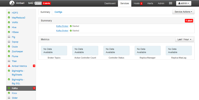
Login to Ambari UI --> Click on Host and add the Kafka Broker to the node where you need to install Broker.

 You can see multiple brokers running in Kafka UI.

 
Step 2: Create a Topic

Login to one of the node where broker is running.  Then create a topic.

cd /usr/iop/4.2.0.0/kafka/bin

su kafka -c "./kafka-topics.sh --create --zookeeper localhost:2181 --replication-factor 2 -partitions 1 --topic CustomerOrder"

You can get the details of the topic using the below describe command.

su kafka -c "./kafka-topics.sh --describe --zookeeper localhost:2181 --topic CustomerOrder"

 
Step 3: Start the Producer

In the argument --broker-list, pass all the brokers that are running.

su kafka -c "./kafka-console-producer.sh --broker-list bi1.test.com:6667,bi2.test.com:6667 --topic CustomerOrder"

When you run the above command, it will be waiting for user input. You can pass a sample message

{"ID":99, "CUSTOMID":234,"ADDRESS":"12,5-7,westmead", "ORDERID":99, "ITEM":"iphone6", "COST":980}

Step 4: Start the Consumer

Open an other Linux terminal and start the consumer. It will display all the messages send to producer.

su kafka -c "./kafka-console-consumer.sh --zookeeper localhost:2181 --from-beginning --topic CustomerOrder"

 

 Thus, We are able to configure and perfom a sample pub-sub system using Kafka.